Introduction

I’ve been working on a video game for some time now. This game has a lot of 2D spacial data I want to query.
But most of this data is sparse, so using a grid would waste a lot of memory.
As an optimization I employed a linear Quadtree. In this post I’ll explore the implementation and provide comparisions with a naive implementation.

All code mentioned in this post will be available on GitHub.

I will use 2*4=8 byte values representing Points and 4 bytes values representing Values. Generalising the data structure will be left to the reader.

What is a Quadtree?

A Quadtree is a data structure to hold 2 dimensional spacial data.

From the Wikipedia page: All forms of quadtrees share some common features:

• They decompose space into adaptable cells
• Each cell (or bucket) has a maximum capacity. When maximum capacity is reached, the bucket splits
• The tree directory follows the spatial decomposition of the quadtree.

Requirements

My use case has the following requirements/characteristics:

• Multiple entities may occupy a position.
• Must be able to query a range.
• Spacial data is updated once per frame. During the execution of a frame the data structure is read-only.
• Positions are represented by integer coordinates (x,y).
• I only plan on supporting x86 architecture at this time.

Naive Quadtree

The bounds of a Node.js will be given as an Axis Aligned Bounding Box (AABB). Represented by their minimum and maximum coordinates.

The quadtree’s body will be a variant of either child nodes or actual values. We will store the actual values in leaf nodes to reduce the number of items we have to probe.
The code of the implementation is available here.

 1
 2
 3
 4
 5
 6
 7
 8
 9
10
11
12
13
14
15
16

// Will store 16 items in a leaf
const LEN_CHILDREN: usize = 16;

#[derive(Debug, Clone)]
pub enum Body {
    Children(Box<[Quadtree; 4]>),
    Items(Box<ArrayVec<[(Point, Value); LEN_CHILDREN]>>),
}

#[derive(Debug, Clone)]
pub struct Quadtree {
    // bounds as an AABB
    from: Point,
    to: Point,
    body: Body,
}

Linear Quadtree

In this implementation I will use a different approach. The data will be stored in dynamic arrays. Points will be sorted by their position in a Z-order curve.
(Re)building is done by inserting all elements, then sorting them by their hash.
I will call this data structure MortonTable

The code of the implementation is available here.

The video demonstrates how the Z-order curve fills the space.

1
2
3
4
5
6

#[derive(Debug, Clone, Default)]
pub struct MortonTable {
    keys: Vec<MortonKey>, // hashed points
    positions: Vec<Point>,
    values: Vec<Value>,
}

Notice how we do not store bounds. This is because this quadtree can operate on the full range of available inputs without them effecting performance. This lets us play with 16 bits per axis = 65,535 ✕ 65,535 grid.

Morton hash

To accomplish this points are hashed using the following routine.
Translated to Rust from Real-Time Collision Detection by Christer Ericson:

 1
 2
 3
 4
 5
 6
 7
 8
 9
10
11
12
13
14
15
16
17

fn morton2(x: u16, y: u16) -> u32 {
    let x = x as u32;
    let y = y as u32;
    partition(x) | (partition(y) << 1)
}

fn partition(mut n: u32) -> u32 {
    // n = ----------------fedcba9876543210 : Bits initially
    // n = --------fedcba98--------76543210 : After (1)
    // n = ----fedc----ba98----7654----3210 : After (2)
    // n = --fe--dc--ba--98--76--54--32--10 : After (3)
    // n = -f-e-d-c-b-a-9-8-7-6-5-4-3-2-1-0 : After (4)
    n = (n ^ (n << 8)) & 0x00ff00ff; // (1)
    n = (n ^ (n << 4)) & 0x0f0f0f0f; // (2)
    n = (n ^ (n << 2)) & 0x33333333; // (3)
    (n ^ (n << 1)) & 0x55555555 // (4)
}

This method is extendable to 32 bit positions with 64 bit keys. This excercise is left to the reader. For my use case 16 bit integer coordinates are more than enough.

Queries

Find value

Finding a value at position is done by finding its hash and returning the Value at the same index, if the tree contains the hash or None otherwise.

Querying a range

Range queries will be done by calculating the minimum and maximum location codes of the AABB of the circle. Then filter this range for points intersecting the circle.

 1
 2
 3
 4
 5
 6
 7
 8
 9
10
11
12
13
14
15
16
17
18
19
20
21
22
23
24
25
26
27
28
29
30

pub fn find_in_range<'a>(
    &'a self,
    center: Point,
    radius: u32,
    out: &mut Vec<(Point, &'a Value)>,
) {
    // calculate the AABB
    let r = r as i32;
    let min = center + Point::new(-r, -r);
    let max = center + Point::new(r, r);

    // find the indices of the minimum and maximum point of the AABB
    // in our values
    let [min, max] = self.morton_min_max(&min, &max);

    // walk the range
    let it = self.positions[min..max]
        .iter()
        .enumerate()
        .filter_map(|(i, id)| {
            // filter the points which intersect the circle
            // and map them to a (point, value) pair
            if center.dist(&id) < radius {
                Some((*id, &self.values[i + min]))
            } else {
                None
            }
        });
    out.extend(it);
}

Walking a range like that will visit a lot of uninteresting points as demonstrated by this video. In this example I have taken a 32✕32 grid and queried a box with coordinates from (10, 12) to (16, 16).
This query will visit 541 points to find the 24 we’re interested in.

Optimizations

On it’s own the linear quadtree isn’t very competitive with the tree implementation. It needs some work to compete with the naive implementation.

Range query splitting

The most important thing I wanted to tackle is reducing the number of “garbage” points when querying a range. To accomplish this we can split the query into multiple sections and query them recursively.
Unfortunately deciding where to split the rectangle is not trivial.
I used the method described here to achive this.
They call the two points that will identify the split as LitMax and BigMin. After identifying these points we will split our original AABB (min, max) to two AABBs (min, litmax) and (bigmin, max).

Note: for most signifact bit (MSB) calculation I’ll use the algorithm described in this paper.
The implementation was taken from this Stack Overflow answer

The algorithm is as follows:

• Identify the most signifact bit that is different between min and max.
• Use that to determine the axis on which to split.
• Calculate the new x1,x2 or y1,y2 positions, depending on the splitting axis.
• Calculate the new location code.

 1
 2
 3
 4
 5
 6
 7
 8
 9
10
11
12
13
14
15
16
17
18
19
20
21
22
23
24
25
26

pub fn litmax_bigmin(
    mortonmin: u32,
    [x1, y1]: [u32; 2],
    mortonmax: u32,
    [x2, y2]: [u32; 2],
) -> [MortonKey; 2] {
    // find the most significant bit that's different
    let diff = mortonmin ^ mortonmax;
    let diff_msb = msb_de_bruijn(diff);

    // split among the side with the higher most significant bit
    // even msb will mean the x axis.
    let [litmax, bigmin] = if diff_msb & 1 == 0 {
        // we compute the diff_msb for both x and y
        // coordinates at the same time
        // this means that msb calculation is done once,
        // but now we have to do a division by 2
        let [x1, x2] = impl_litmax_bigmin(x1, x2, diff_msb / 2);
        // we inherit the Y coordinates from the original points
        // note that they have been flipped!
        [MortonKey::new_u32(x1, y2), MortonKey::new_u32(x2, y1)]
    } else {
        // pretty much the same as above but x and y are swapped
    };
    [litmax, bigmin]
}

Producing the new coordinates is done by:

• Take the shared most significant bits as prefix.
• Produce the max suffix by setting the most significant different bit to 1 and the less significant bits to 0.
• Subtract 1 for the min suffix.
• Merge the prefix with each suffix respectively.

Take for example a = 0b1100101 and b = 0b1101100

• The most significant different bit is the 4th.
• Produce the following prefix: 0b1100000
• Suffix 2 will be 0b1000
• Subtracting 1 gives 0b0111
• Interleaving the prefix with the suffixes yields 0b1101000 and 0b1100111

 1
 2
 3
 4
 5
 6
 7
 8
 9
10
11
12
13
14
15
16
17

/// `diff_msb`: position of the most significant bit
/// that's different between `a` and `b`
fn impl_litmax_bigmin(a: u32, b: u32, diff_msb: u32) -> [u32; 2] {
    let prefix2 = 1 << diff_msb;
    let prefix1 = prefix2 - 1;

    // calculate the common most significant bits
    // aka. the prefix
    let mask = !(!prefix2 & prefix1);
    let z = (a & b) & mask;
    // append the suffixes
    let litmax = z | prefix1;
    let bigmin = z | prefix2;

    [litmax, bigmin]
}

So now that we can split queries to reduce the number of elements we have to visit, but when should we split? The original paper split after 3 garbage points. When benchmarking I found that instead splitting based on the number of elements left to visit was more benecitial.

 1
 2
 3
 4
 5
 6
 7
 8
 9
10
11
12
13
14
15
16
17
18
19
20
21
22
23
24
25
26
27
28
29
30
31
32
33
34
35
36
37
38
39
40
41
42
43
44
45
46
47
48

fn find_in_range_impl<'a>(
    &'a self,
    center: &Point,
    radius: u32,
    min: MortonKey,
    max: MortonKey,
    out: &mut Vec<(Point, &'a Value)>,
) {
    // `find_key_morton` finds the index of the key provided,
    // or returns the index the key would have to be inserted
    // to keep the keys sorted.
    let (imin, pmin) = self
        .find_key_morton(&min)
        .map(|i| (i, *self.positions[i]))
        .unwrap_or_else(|i| (i, min.as_point()));

    let (imax, pmax) = self
        .find_key_morton(&max)
        // add 1 to include this node in the range query as otherwise
        // an element might be missed
        .map(|i| (i + 1, *self.positions[i]))
        .unwrap_or_else(|i| (i, max.as_point()));

    if imax < imin {
        return;
    }

    // The original paper counts the garbage items
    // and splits above a threshold.
    // Instead let's speculate if we need a split or
    // if it more beneficial to just scan the range.
    // The number I picked is more or less arbitrary,
    // it is a power of two and I ran the basic
    // benchmarks to probe a few numbers.
    if imax - imin > 16 {
        let [litmax, bigmin] = litmax_bigmin(min.0, pmin, max.0, pmax);
        // split and recurse
        self.find_in_range_impl(center, radius, min, litmax, out);
        self.find_in_range_impl(center, radius, bigmin, max, out);
        return;
    }

    for (i, id) in self.positions[imin..imax].iter().enumerate() {
        if center.dist(&id) < radius {
            out.push((*id, &self.values[i + imin]));
        }
    }
}

Once we apply this change to the query above it will split to 11 sub-queries, visiting 48 nodes, of which 13 will be garbage.
The original query visits 541 points. One can play with the threshold we split at, I found 16 to be a good trade-off between the allowed garbage and the number of splits.

In the COTS dynamic POIs paper the authors were counting “misses” when querying elements and splitting at 3.
I found that splitting when the scan-range is above a threshold (32) results in about 30% increase in performance, even tough we visit more garbage.
This is most likely because we better utilize the branch preditor of the CPU.
As a rule of thumb you should avoid conditionals in loops as much as you can to better utilize branch prediction in your code.

Here’s a demonstration of the same query as above, using recursive splitting to cut down the visited range.

Skiplist

When you pull in data from a the L3 cache or memory, querying it is basically free.

When we search for the index of a key we need to pull the vector of hashes into the L1 cache. This means that from the typical 64 byte long L1 cache line only 24 (size of a Vec) will be used.
(Actually I use only 16 bytes, the beginning and ending pointer, but Vec bundles the begin,end and capacity pointers in one).
We can improving performance by placing some keys into this memory space, that is already in the cache anyway.

We’ll build a skip-list to divide the full range of hashes to 8 buckets.
This let’s us cut down the range we actually have to probe by a factor of 8, before pulling the actual memory we probe from memory!

 1
 2
 3
 4
 5
 6
 7
 8
 9
10
11
12
13

const SKIP_LEN: usize = 8;
type SkipList = [u32; SKIP_LEN];

#[derive(Debug, Clone, Default)]
pub struct MortonTable {
    skipstep: u32,
    skiplist: SkipList,
    // ---- 9 * 4 bytes so far
    // `keys` is 24 bytes in memory
    keys: Vec<MortonKey>,
    positions: Vec<Point>,
    values: Vec<Value>,
}

Rebuilding the skip-list is done by dividing keys to 8 buckets and saving the hash at the beginning of each bucket (skipping the first).

 1
 2
 3
 4
 5
 6
 7
 8
 9
10
11
12
13
14
15
16
17
18
19
20
21
22

fn rebuild_skip_list(&mut self) {
    let len = self.keys.len();
    let step = len / SKIP_LEN;
    self.skipstep = step as u32;
    if step == 0 {
        // We have less than 8 elements
        // Optimization opportunity: in this case store all hashes in the skiplist!
        if let Some(key) = self.keys.last() {
            // We have more than 0 elements
            self.skiplist[0] = key.0;
        }
        return;
    }
    for (i, k) in (0..len)
                .step_by(step) // take ints 0, step, 2*step ...
                .skip(1) // skip the first (0)
                .take(SKIP_LEN) // take SKIP_LEN=8 at maximum
                .enumerate() // return the index of the current item (i)
    {
        self.skiplist[i] = self.keys[k].0;
    }
}

Now the fun part: looking up the bucket where a hash may reside.
I’ll use SSE extensiont to find the bucket I’ll have to probe later.

 1
 2
 3
 4
 5
 6
 7
 8
 9
10
11
12
13
14
15
16
17
18
19
20
21
22
23
24
25

/// Find the index of the partition `key` may be found.
/// (little bit simplified for the blog post)
unsafe fn find_key_partition_sse2(
    // skiplist
    [s0, s1, s2, s3]: &[i32; 4],
    key: i32
) -> usize {
    // create a vector of 4 of the key
    let keys4 = _mm_set_epi32(key, key, key, key);

    // create two 128 bit vectors from the 8 skip-list values.
    let skiplist: __m128i = _mm_set_epi32(s0, s1, s2, s3);

    // set every 32 bits to 0xFFFF if key < skip else set it to 0x0000
    let results: __m128i = _mm_cmpgt_epi32(keys4, skiplist);

    // create a mask from the most significant bit of each 8bit element
    let mask: i32 = _mm_movemask_epi8(results);

    // count the number of bits set to 1
    let count: i32 = _popcnt32(mask);
    // because the mask was created from 8 bit wide items
    // every key in the skip list is counted 4 times.
    count as usize / 4
}

Once the bucket is found I’ll use binary search to find the position of the key.

Because x86 only supplies signed 32 bit comparisions, I choose to reduce the available coordinate domain to 15 bits to avoid problems with the sign bit.
This still provides an available grid of 32,768 ✕ 32,768 = 1,073,741,824 points, more than enough for my use case.
The reader might take another approach based on their problem domain, for example using 8bit comparisions.

Benchmarks

Benchmarks are the only source of truth you’ll ever get, and they are lies. Every last one of them.

Before we begin note the above quote by Matt Kulukundis and keep in the back of your mind.

For benchmarking I’ll use the Criterion framework.
Criterion will always warm up the cache, so all benchmarks are taken with hot caches.
This means that these benchmarks might not be applicable for your use case.
Also besides the absolute value of savings we make it is also important to count how many times that functionality is used.
For example, if I save 1 micro seconds in a 16ms frame that won’t be noticable. But if I save 1 micro seconds on a function that is called a million times, then I saved 1 seconds of runtime.

The raw report produced is available here.
For the benchmarks I use a large amount of random, so I use the same seed for every run.

Notes:

• 1 us == 1000 ns
• 1 ms == 1000 us
• 1 s == 1000 ms
• Lower is better.

Querying a range

For this benchmark I build a tree with points in range of (0, 7800) for sparse, and (0, 400) for dense experiments.
Then I’ll run range queries with random centers and fixed, (512 for dense, and 50 for sparse) radius.
The naive quadtrees will be built using from_iterator which will find the minimum bounding box the points occupy, so it should be well balanced.
The grids are squares.

After applying this optimization the linear quadtree beats the naive implementation by a substantial amount.

Experiment MortonTable_counting_misses uses a find_in_range implementation that counts the outlying points visited when querying and splits when the query encounters 3 outliers.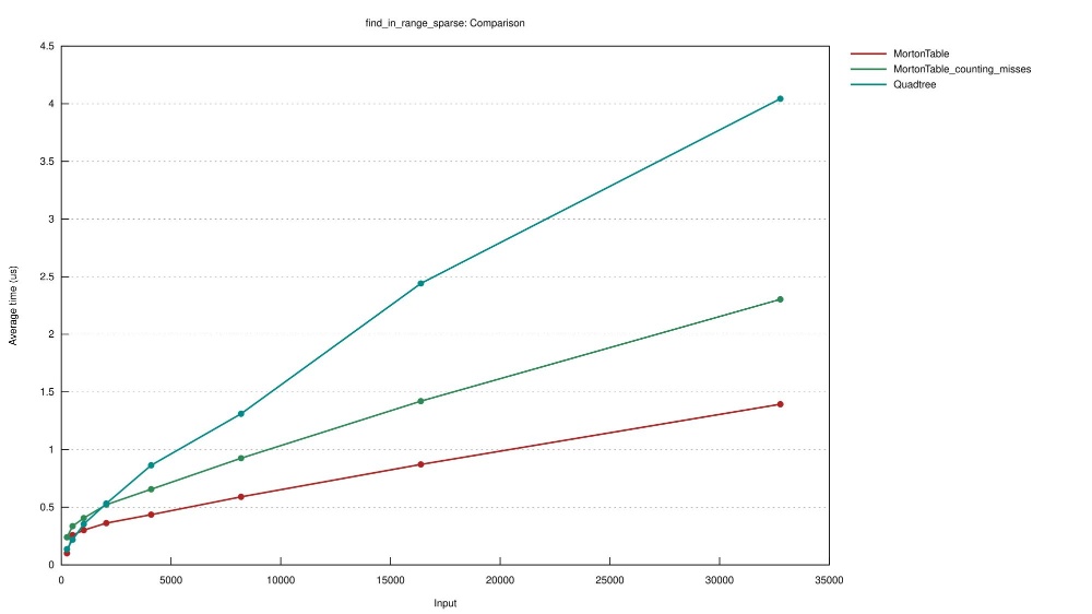

So at 32.7 thousand sparsely placed points, the MortonTable performs about 13 times better.

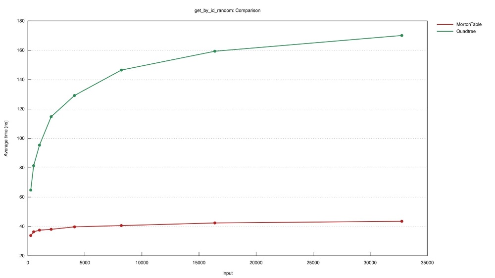
Querying a single point

Measure the time to check wether the given point was inserted into the tree, without returning its actual Value.
For this benchmark I’ll build trees from points spanning the range (0, 7800) and then query random points.

Contains

Experiment contains_rand will check if the tree contains a given point.
Experiment get_by_id_random will query a single value at a given position.
Experiment get_by_id_random_in_table will query a single value at points that are guaranteed to be in the table.

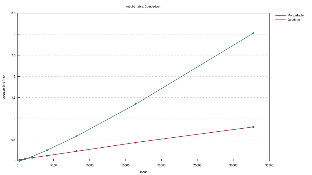
Rebuilding

Experiment make_table measures the time it takes to build a tree from the group up.
Experiment rebuild_table measures the time it takes to clear and rebuild a tree, reusing the existing data structure.

The reader should observe that for small inputs Quadtree building is faster than MortonTable but it will turn around quickly.

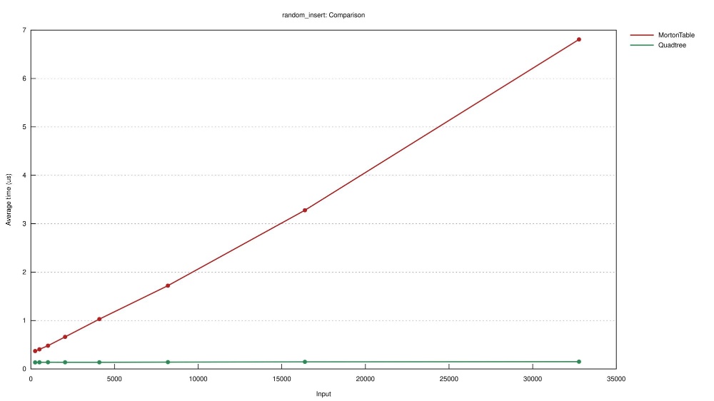
Inserting

So far the MortonTable outperformes Quadtree in most benchmarks. But whenever you do programming, and especially performance work there are trade-offs to make.
The trade-off we make here is in the insertion and deletion time of single elements. Because our lists need to be sorted, random insertion (and deletion) has a huge cost.
As you can see in the table below, this MortonTable implementation is useless if you need on demand insertions and deletions.

If you do need on-demand insert/delete you could swap out the keys Vec to a HashMap<MortonKey, usize> where the values are the indices of items in the storage vectors.
Now you could delete by swapping with the last item and insert by appending.
This would mean that the order of the values will be mixed up, when running range queries you’ll jump around in memory more to find the values.
Meaning worse cache utilization.
I suspect this would be very bad for find_in_range, so this is not an easy trade-off to make.

Final thoughts

Building efficient data structures requires you know your problem domain so you can choose the trade-offs you make. There is no silver bullet, you will have to choose trade-offs to make.
When optimizing it is a good practice to start with algorithmic improvements and then move on to architectural optimizations.